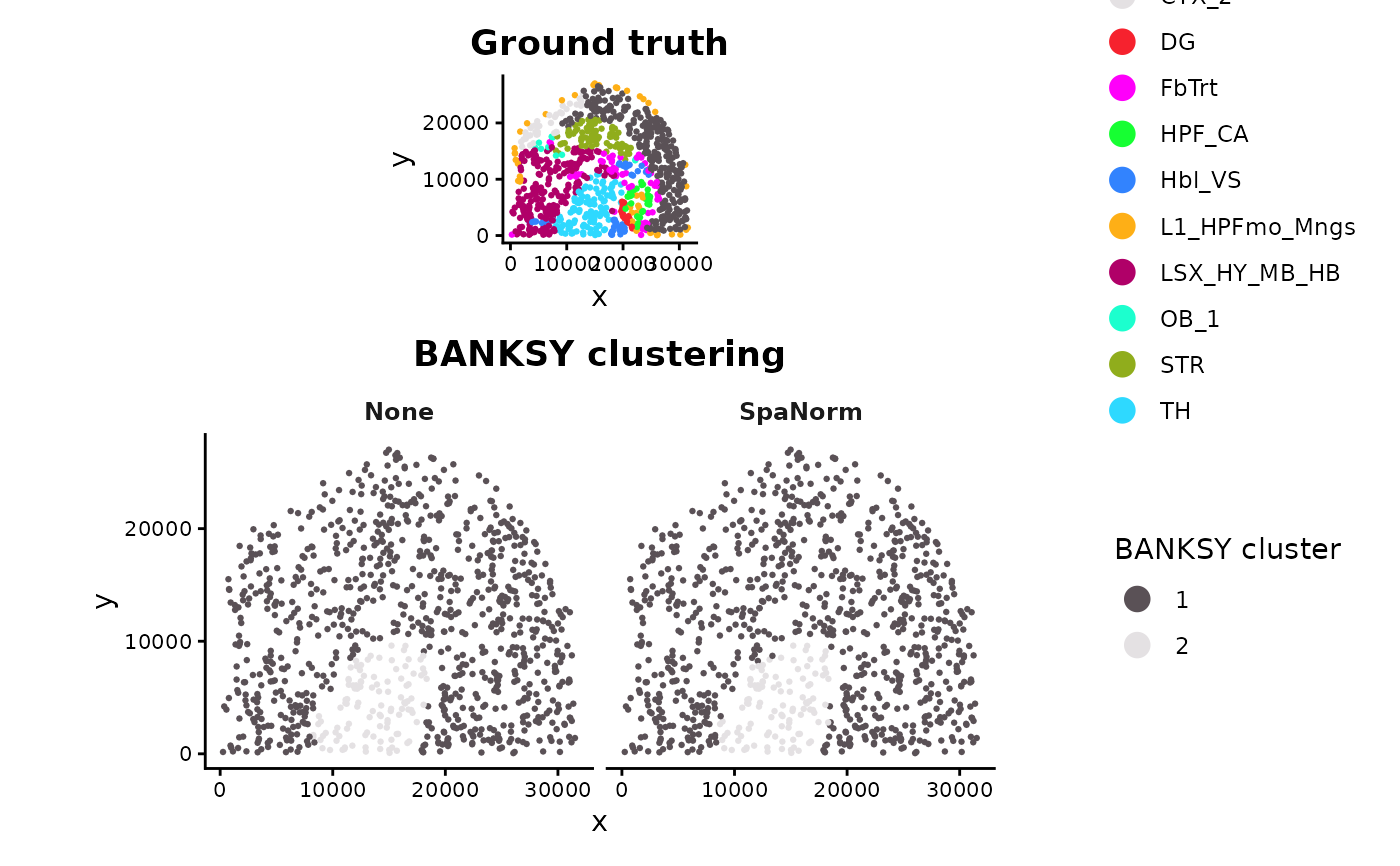
Visualise predicted spatial clusters and ground-truth annotations across normalisation methods.
Arguments
- norm_list
Named list of SpatialExperiment objects or nested lists of SpatialExperiment objects.
- cluster_col
Column containing predicted clusters.
- methods
Optional normalisation methods to plot.
- method_order
Optional method order.
- point_size
Spatial point size.
- palette
Optional named colours for predicted clusters.
- ncol
Number of columns for spatial facets.
- legend_point_size
Point size in legends.
- theme_name
Plot theme.
- ground_truth_col
Ground-truth annotation column.
- show
One of "both", "predicted", or "truth".
- truth_palette
Optional named colours for ground truth.
Details
When show = "both", the ground truth is displayed once per spatial slice, followed by predicted cluster maps across all selected normalisation methods.
Predicted clusters share one colour scale and legend. Ground truth uses a separate palette and legend.
Examples
data(norm_example)

banksy_norm <- run_banksy_individual(
  norm_list = norm_example,
  k_geom = 15,
  lambda = 0.8,
  resolution = 0.2,
  seed = 123
)
#> Computing neighbors...
#> Spatial mode is kNN_median
#> Parameters: k_geom=15
#> Done
#> Done
#> Using seed=123
#> Using seed=123
#> Computing neighbors...
#> Spatial mode is kNN_median
#> Parameters: k_geom=15
#> Done
#> Done
#> Using seed=123
#> Using seed=123

p <- plot_spatial_clustering(
  norm_list = banksy_norm,
  cluster_col = "banksy_cluster",
  ground_truth_col = "layer_guess",
  show = "both",
  point_size = 0.5,
  ncol = 2,
  theme_name = "classic"
)

p$plot