Cell-type annotation and spatial clustering with STBench
Source:vignettes/annotation-and-clustering.Rmd
annotation-and-clustering.RmdIntroduction
This vignette uses the cell-type labels already supplied in
norm_example, so an external SingleR reference is not
required.
Cell-type annotation
The example data include existing cell_type annotations.
We use these to demonstrate downstream comparisons without requiring an
external SingleR reference. In a full analysis,
run_annotation() can be used with an appropriate
reference.
annotated_norm <- norm
annotation_col <- "cell_type"
Visualise spatial cell-type assignments
p_annotation <- plot_spatial_annotation(
  norm_list = annotated_norm,
  annotation_col = annotation_col,
  method_order = NULL,
  point_size = 0.5,
  ncol = 2,
  theme_name = "classic",
  palette = "turbo"
)
p_annotation$plot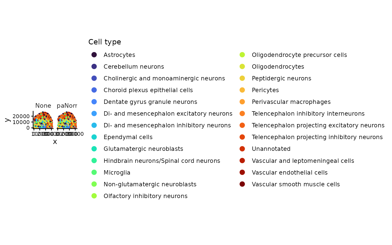
Compare cell-type composition
We examine relative proportions and absolute spot counts assigned to each cell type.
p_prop <- plot_celltype_proportion(
  norm_list = annotated_norm,
  annotation_col = annotation_col,
  palette = "turbo",
  show = "proportion",
  theme_name = "classic"
)
p_prop$plot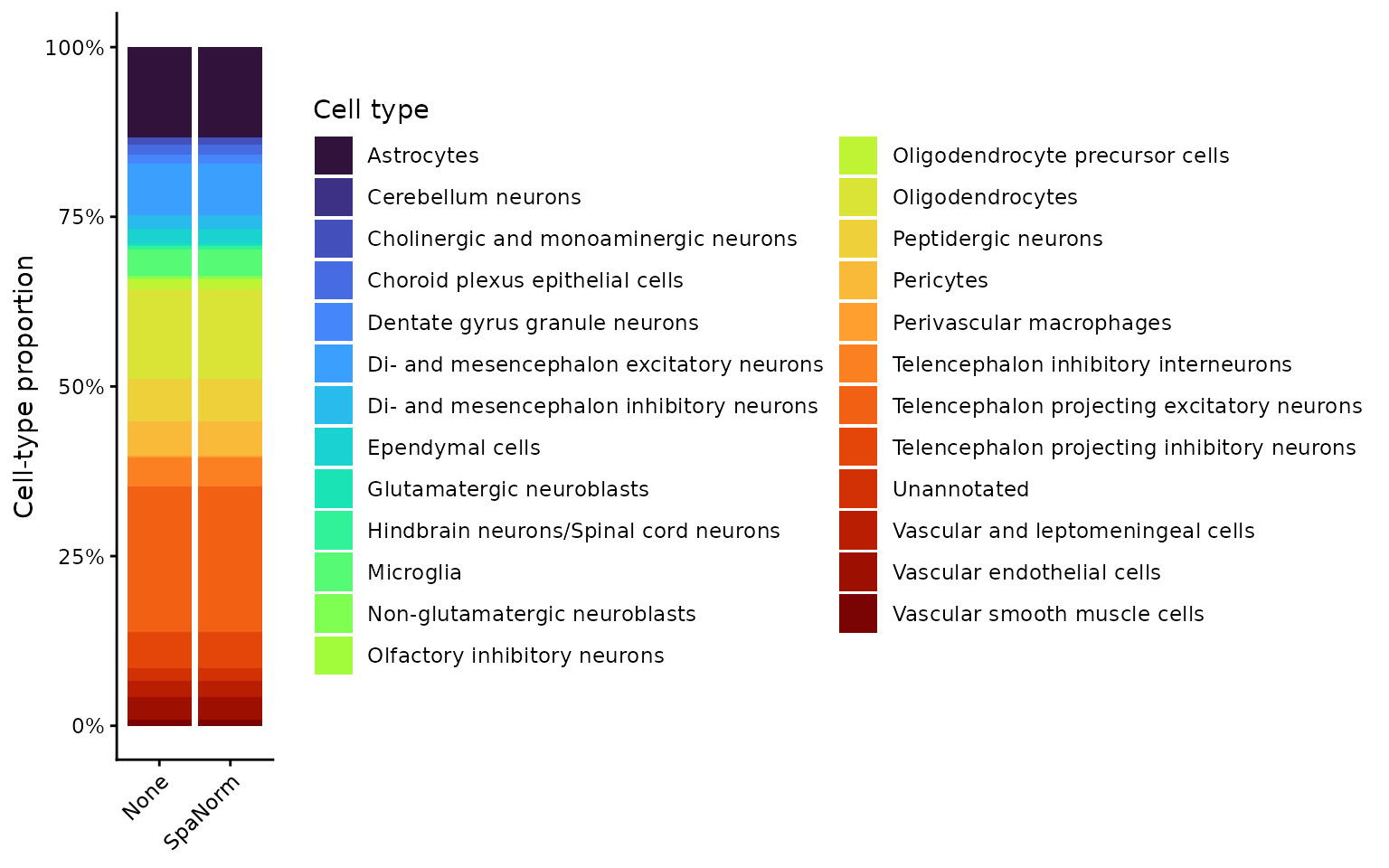
p_count <- plot_celltype_proportion(
  norm_list = annotated_norm,
  annotation_col = annotation_col,
  show = "count",
  theme_name = "classic"
)
p_count$plot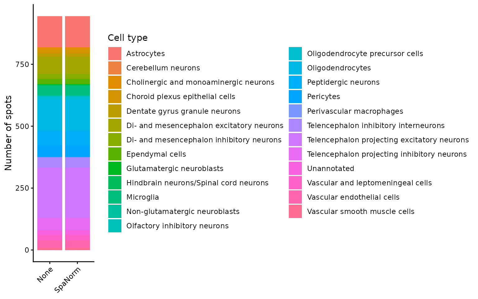
Calculate and plot annotation agreement
Pairwise agreement measures the fraction of spots receiving the same label under two methods. It measures consistency, not accuracy against a known ground truth.
annotation_agreement <- calculate_annotation_agreement(
  norm_list = annotated_norm,
  annotation_col = annotation_col,
  remove_na = TRUE
)
annotation_agreement
#>   method1 method2 agreement n_compared
#> 1    None SpaNorm         1        944

p_agreement <- plot_annotation_agreement(
  norm_list = annotated_norm,
  annotation_col = annotation_col,
  remove_na = TRUE,
  show_values = TRUE,
  digits = 2,
  colour_option = "viridis",
  theme_name = "classic"
)
p_agreement$plot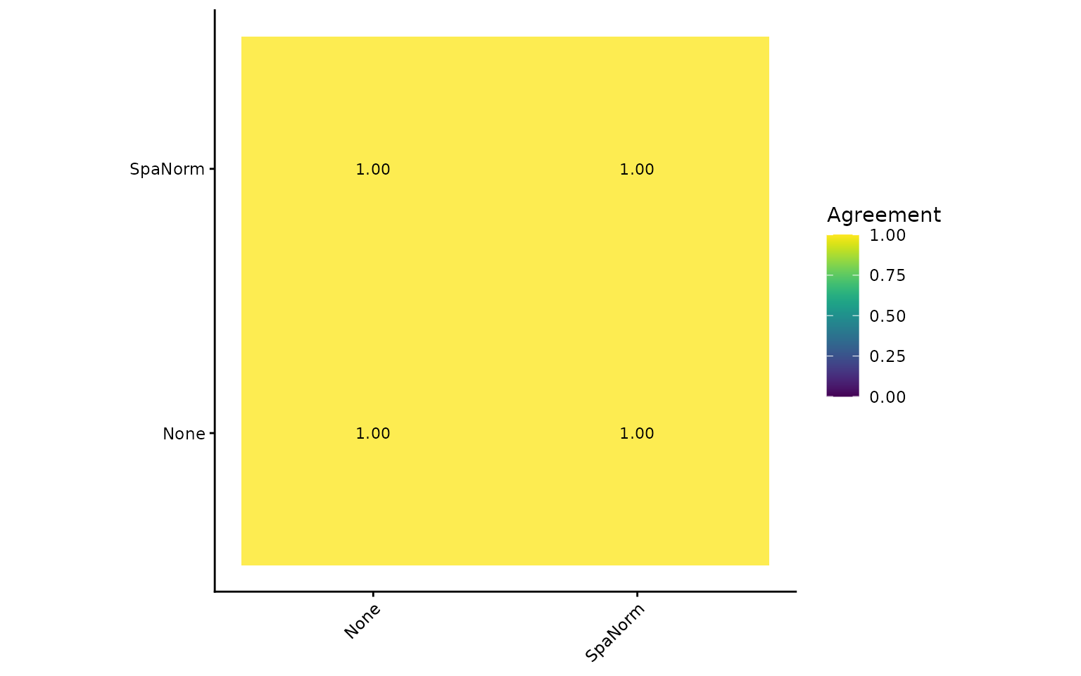
Marker investigations
Marker comparisons depend on the presence of biologically relevant genes. The following code demonstrates how to specify candidate markers when available.
p_marker <- plot_marker_expression(
  norm_list = annotated_norm,
  markers = head(rownames(annotated_norm[[1]]), 2),
  annotation_col = "cell_type",
  palette = "turbo"
)
p_marker$plot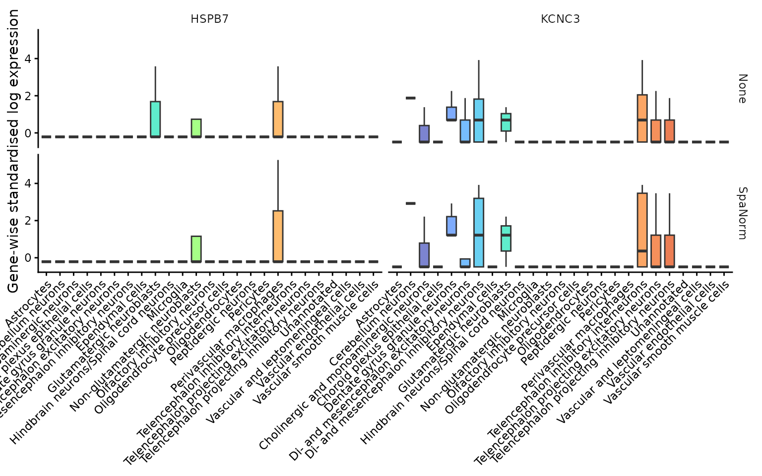
BANKSY spatial clustering
BANKSY incorporates spatial neighbourhood information alongside gene expression to identify spatial domains. We execute clustering on the small example dataset.
banksy_norm <- run_banksy_individual(
  norm_list = norm,
  methods = names(norm),
  assay_name = "logcounts",
  cluster_col = "banksy_cluster",
  k_geom = 15,
  lambda = 0.8,
  resolution = 0.2,
  seed = 123
)
Visualise and evaluate BANKSY clusters
These functions operate on the output of
run_banksy_individual() above.
p_banksy <- plot_spatial_clustering(
  norm_list = banksy_norm,
  cluster_col = "banksy_cluster",
  ground_truth_col = "layer_guess",
  show = "both",
  methods = names(banksy_norm),
  point_size = 0.5,
  ncol = 2,
  theme_name = "classic"
)
p_banksy$plot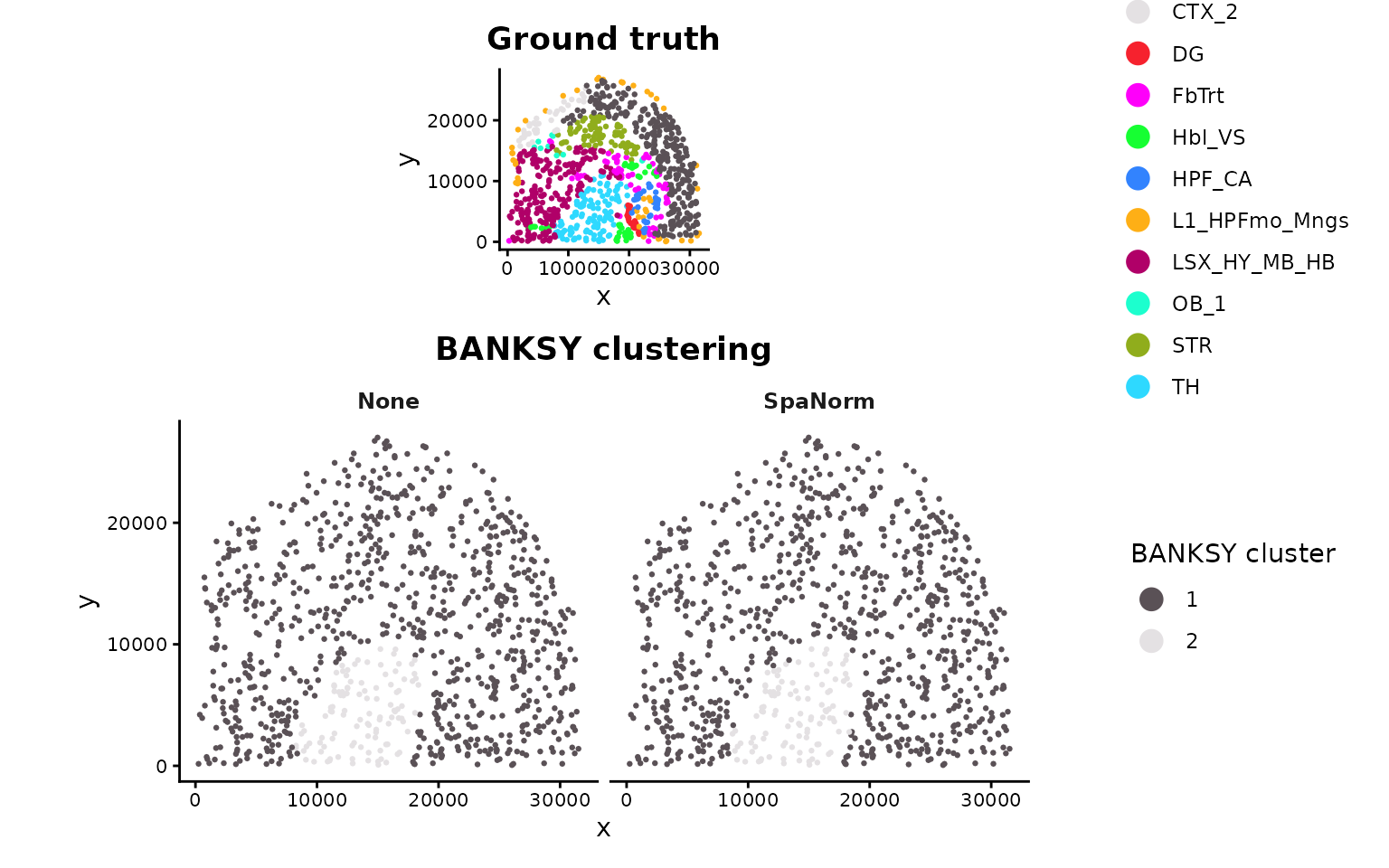
metrics_df <- calculate_clustering_metrics(
  norm_list = banksy_norm,
  ground_truth_col = "layer_guess",
  cluster_col = "banksy_cluster",
  methods = names(banksy_norm)
)
metrics_df
#>    method  slice   n        ARI       NMI       HOM       COM          ASW
#> 1    None slice1 944 0.08916554 0.2532399 0.1489408 0.8449019  0.004987321
#> 2 SpaNorm slice1 944 0.08558020 0.2423588 0.1421474 0.8215048 -0.002514273
#>     Overall n_asw ASW_sampled
#> 1 0.4156942   944       FALSE
#> 2 0.4020037   944       FALSE

p_metrics <- plot_clustering_metrics(
  metrics_df = metrics_df,
  metrics = c("ARI", "NMI", "HOM", "COM", "ASW", "Overall"),
  ncol = 2,
  scales = "free_y",
  theme_name = "bw"
)
p_metrics$plot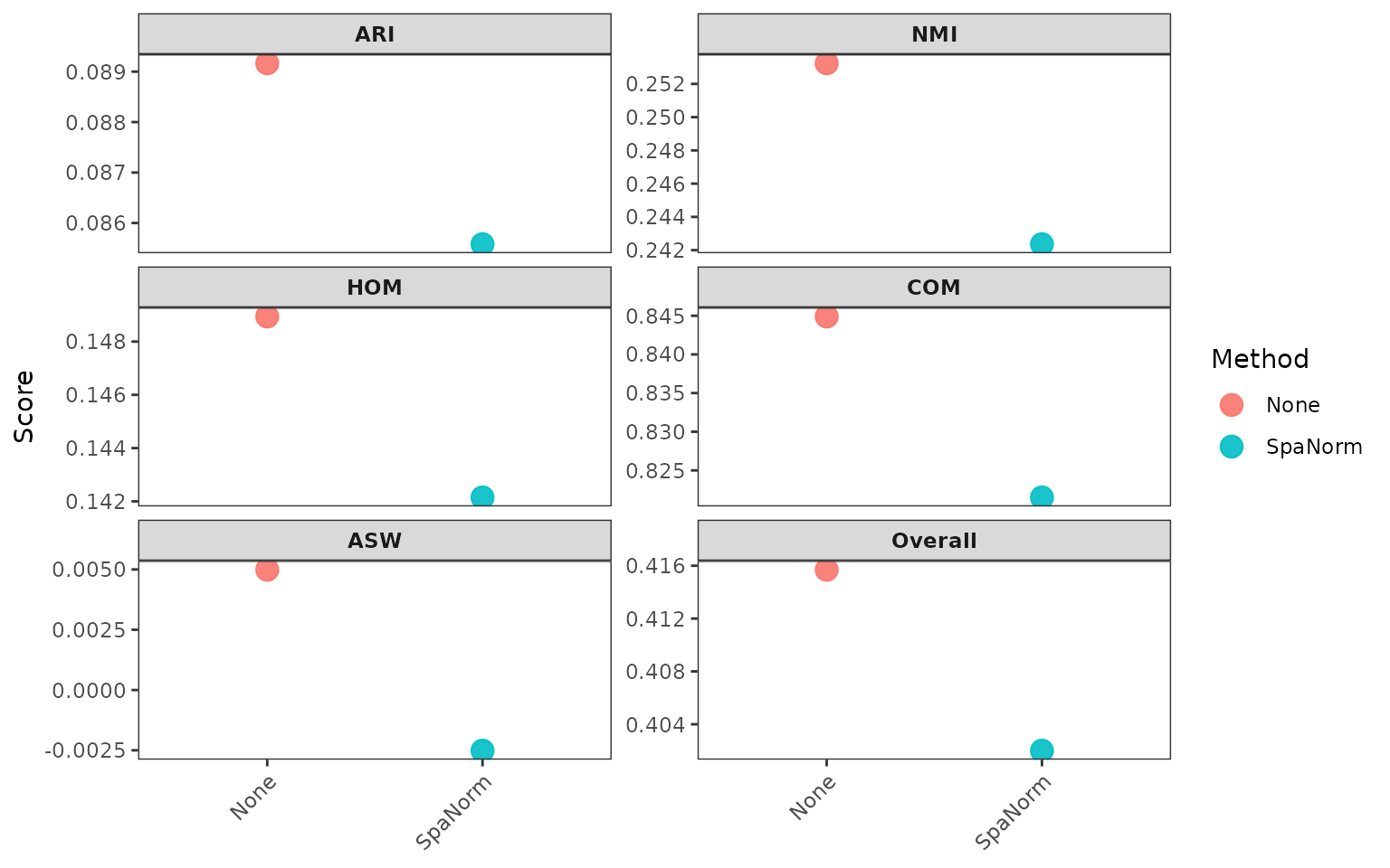
ranking_df <- rank_normalization_methods(metrics_df = metrics_df)
ranking_df
#>   Rank  method   Overall
#> 1    1    None 0.4156942
#> 2    2 SpaNorm 0.4020037

p_ranking <- plot_normalization_ranking(
  ranking_df = ranking_df,
  bar_width = 0.7,
  label_size = 3.5,
  theme_name = "classic"
)
p_ranking$plot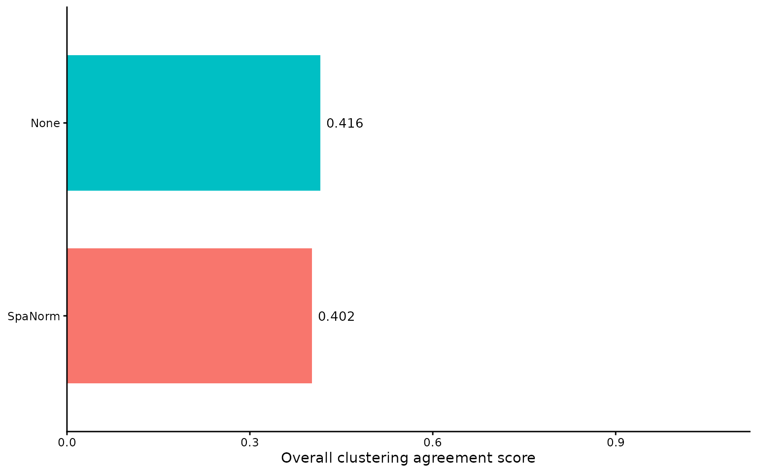
BANKSY with different gene-selection strategies
For a small example dataset, a selection size of 500 can exceed the number of available genes. For the small dataset, each selection strategy uses up to the available number of genes.
data(svg_example)

banksy_genes <- run_banksy_gene_selection(
  norm_list = norm,
  svg_list = svg_example,
  gene_selection = "all",
  assay_name = "logcounts",
  k_geom = 15,
  lambda = 0.8,
  resolution = 0.2,
  seed = 123
)

metrics_genes <- calculate_gene_selection_metrics(
  banksy_list = banksy_genes,
  ground_truth_col = "layer_guess"
)

p_genes <- plot_gene_selection_metrics(
  metrics_df = metrics_genes,
  ncol = 3,
  scales = "free_y",
  theme_name = "classic"
)
p_genes$plot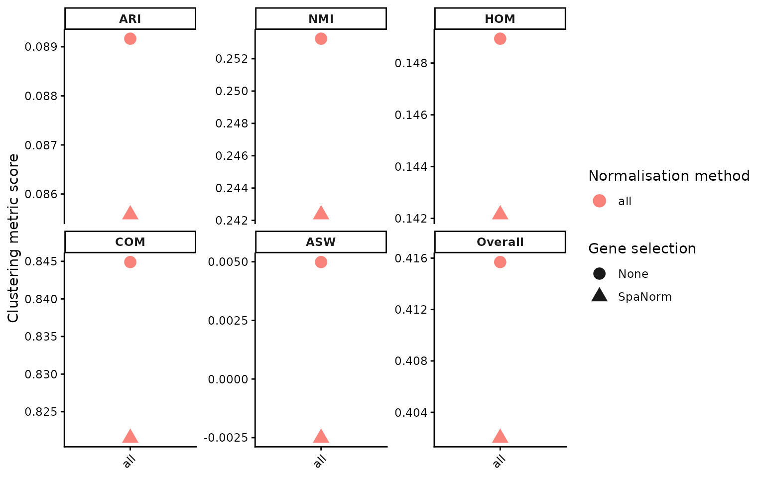
Session information
sessionInfo()
#> R version 4.5.0 (2025-04-11)
#> Platform: x86_64-pc-linux-gnu
#> Running under: Red Hat Enterprise Linux 9.8 (Plow)
#>
#> Matrix products: default
#> BLAS/LAPACK: FlexiBLAS OPENBLAS;  LAPACK version 3.10.1
#>
#> locale:
#>  [1] LC_CTYPE=en_AU.UTF-8       LC_NUMERIC=C
#>  [3] LC_TIME=en_AU.UTF-8        LC_COLLATE=en_AU.UTF-8
#>  [5] LC_MONETARY=en_AU.UTF-8    LC_MESSAGES=en_AU.UTF-8
#>  [7] LC_PAPER=en_AU.UTF-8       LC_NAME=C
#>  [9] LC_ADDRESS=C               LC_TELEPHONE=C
#> [11] LC_MEASUREMENT=en_AU.UTF-8 LC_IDENTIFICATION=C
#>
#> time zone: Australia/Melbourne
#> tzcode source: system (glibc)
#>
#> attached base packages:
#> [1] stats     graphics  grDevices utils     datasets  methods   base
#>
#> other attached packages:
#> [1] STBench_0.99.0
#>
#> loaded via a namespace (and not attached):
#>  [1] tidyselect_1.2.1            viridisLite_0.4.3
#>  [3] dplyr_1.2.0                 farver_2.1.2
#>  [5] viridis_0.6.5               S7_0.2.1
#>  [7] fastmap_1.2.0               SingleCellExperiment_1.32.0
#>  [9] digest_0.6.39               lifecycle_1.0.5
#> [11] cluster_2.1.8.2             magrittr_2.0.4
#> [13] dbscan_1.2.4                compiler_4.5.0
#> [15] rlang_1.1.7                 sass_0.4.10
#> [17] tools_4.5.0                 igraph_2.2.2
#> [19] yaml_2.3.12                 data.table_1.18.2.1
#> [21] knitr_1.51                  S4Arrays_1.9.1
#> [23] labeling_0.4.3              htmlwidgets_1.6.4
#> [25] scatterplot3d_0.3-45        mclust_6.1.2
#> [27] DelayedArray_0.35.2         RColorBrewer_1.1-3
#> [29] abind_1.4-8                 withr_3.0.3
#> [31] purrr_1.2.1                 BiocGenerics_0.56.0
#> [33] desc_1.4.3                  grid_4.5.0
#> [35] stats4_4.5.0                colorspace_2.1-2
#> [37] aricode_1.1.0               ggplot2_4.0.2
#> [39] scales_1.4.0                dichromat_2.0-0.1
#> [41] SummarizedExperiment_1.39.1 cli_3.6.5
#> [43] rmarkdown_2.31              crayon_1.5.3
#> [45] ragg_1.4.0                  leidenAlg_1.1.5
#> [47] generics_0.1.4              otel_0.2.0
#> [49] rstudioapi_0.17.1           rjson_0.2.23
#> [51] Banksy_1.5.6                cachem_1.1.0
#> [53] RcppHungarian_0.3           parallel_4.5.0
#> [55] XVector_0.49.0              matrixStats_1.5.0
#> [57] vctrs_0.7.2                 Matrix_1.7-4
#> [59] jsonlite_2.0.0              clevr_0.1.2
#> [61] patchwork_1.3.2             IRanges_2.43.0
#> [63] S4Vectors_0.47.0            irlba_2.3.7
#> [65] systemfonts_1.3.1           magick_2.9.1
#> [67] jquerylib_0.1.4             tidyr_1.3.2
#> [69] glue_1.8.1                  pkgdown_2.2.1
#> [71] uwot_0.2.4                  Polychrome_1.6.1
#> [73] gtable_0.3.6                GenomicRanges_1.61.1
#> [75] tibble_3.3.1                pillar_1.11.1
#> [77] htmltools_0.5.9             Seqinfo_0.99.2
#> [79] R6_2.6.1                    textshaping_1.0.1
#> [81] evaluate_1.0.5              sccore_1.0.6
#> [83] lattice_0.22-9              Biobase_2.69.0
#> [85] SpatialExperiment_1.20.0    bslib_0.10.0
#> [87] Rcpp_1.1.1                  gridExtra_2.3
#> [89] SparseArray_1.9.0           xfun_0.57
#> [91] fs_1.6.6                    MatrixGenerics_1.22.0
#> [93] pkgconfig_2.0.3