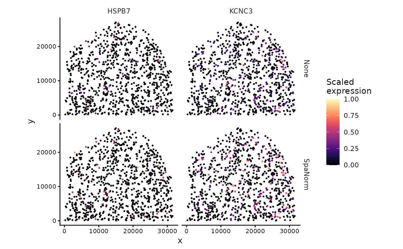
Plot spatial expression across normalisation methods
Source:R/svg_expression.R
plot_spatial_expression.RdVisualise spatial expression of selected genes across multiple normalisation methods.
Usage
plot_spatial_expression(
  norm_list,
  genes,
  assay_name = "logcounts",
  method_order = NULL,
  scale_expr = TRUE,
  point_size = 0.5,
  colour_option = "magma",
  ncol_genes = 1,
  theme_name = "classic",
  methods = NULL,
  scale_by = c("gene", "gene_method")
)
Arguments
- norm_list
Named list of normalised SpatialExperiment objects.
- genes
Character vector of genes to plot.
- assay_name
Name of the expression assay.
- method_order
Optional ordering of selected methods.
- scale_expr
Logical. Whether to scale expression.
- point_size
Spatial point size.
- colour_option
Viridis colour option.
- ncol_genes
Number of columns for unscaled plots.
- theme_name
Plot theme.
- methods
Optional character vector of normalisation methods. If NULL, all available methods are used.
- scale_by
Scaling approach: "gene" or "gene_method".
Details
Expression can be scaled between 0 and 1 either across all selected methods for each gene or independently within each gene and normalisation method.
When scale_expr = FALSE, original assay values are used. Each gene receives a separate plot with a common colour scale across the selected methods.
Examples
data(norm_example)

genes <- head(rownames(norm_example[[1]]), 2)

p_expr <- plot_spatial_expression(
  norm_list = norm_example,
  genes = genes,
  assay_name = "logcounts",
  scale_expr = TRUE,
  scale_by = "gene",
  point_size = 0.5,
  colour_option = "magma",
  ncol_genes = 1,
  theme_name = "classic"
)

p_expr$plot