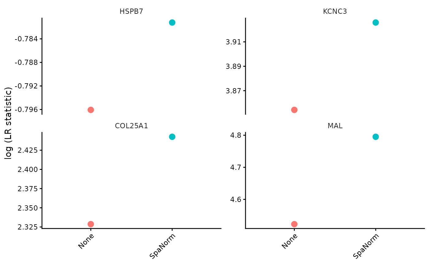
Plot distributions of spatial variability statistics for multiple user-defined gene sets across normalisation methods.
Usage
plot_svg_gene_sets(
  svg_norm,
  gene_sets,
  stat = "LR_stat",
  method_order = NULL,
  method_colors = NULL,
  gene_id = "rownames",
  transform = c("log1p", "log", "none"),
  plot_type = c("boxplot", "violin"),
  scales = c("free_y", "fixed", "free"),
  facet_ncol = 2,
  add_jitter = TRUE,
  point_size = 1,
  alpha = 0.65,
  jitter_alpha = 0.5,
  box_width = 0.65,
  title = NULL,
  subtitle = NULL,
  x_label = "Normalisation method",
  y_label = NULL,
  show_legend = FALSE,
  theme_name = "classic"
)
Arguments
- svg_norm
Named list of SVG results.
- gene_sets
Named list of character vectors containing genes for each gene set.
- stat
SVG statistic. Default is "LR_stat".
- method_order
Optional normalisation method order.
- method_colors
Optional named vector of method colours.
- gene_id
Gene identifier.
- transform
Transformation: "log1p", "log", or "none".
- plot_type
Plot type: "boxplot" or "violin".
- scales
Facet scales: "fixed", "free_y", or "free".
- facet_ncol
Number of facet columns.
- add_jitter
Logical. Display individual gene points.
- point_size
Size of jittered points.
- alpha
Transparency of boxplots or violins.
- jitter_alpha
Transparency of jittered points.
- box_width
Width of boxplots.
- title
Optional plot title.
- subtitle
Optional plot subtitle.
- x_label
X-axis label.
- y_label
Optional y-axis label.
- show_legend
Logical. Display method legend.
- theme_name
Plot theme.
Details
Gene sets may include housekeeping genes, negative-control genes, biological marker genes, or any custom gene sets.
Each gene set is displayed in a separate facet.
Examples
data(svg_example)

marker_genes <- head(rownames(svg_example[[1]]), 5)

p <- plot_svg_stat(
  svg_norm = svg_example,
  genes = marker_genes,
  stat = "LR_stat",
  transform = "log"
)

p$plot