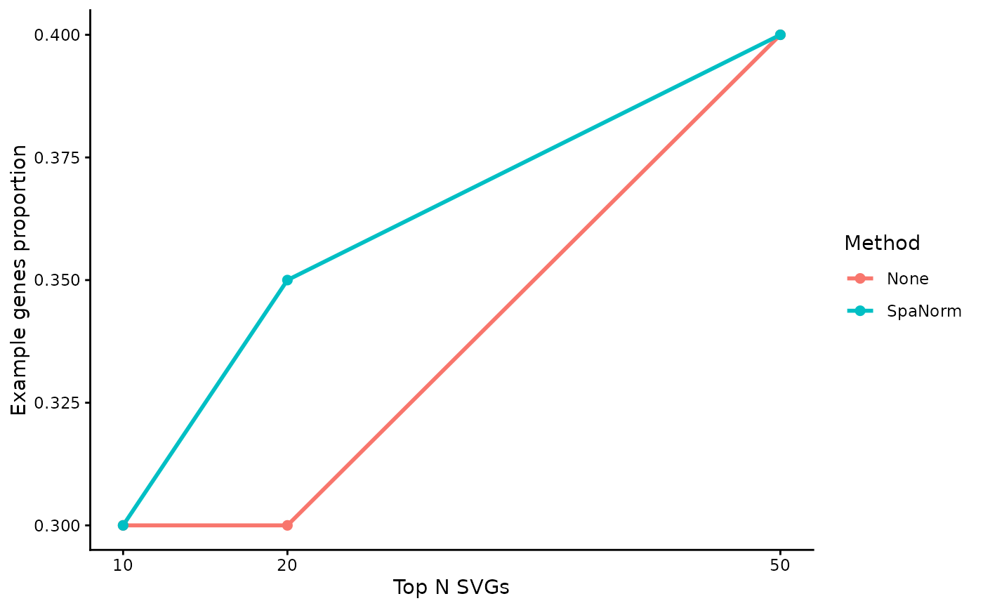
Calculate and visualise the proportion of genes belonging to a user-defined gene set among the top-ranked spatially variable genes (SVGs) across normalisation methods.
Usage
plot_svg_topn_gene_set(
  svg_norm,
  genes,
  top_n = c(50, 100, 200, 300),
  method_order = NULL,
  method_colors = NULL,
  gene_id = "rownames",
  theme_name = "classic",
  gene_set_name = "Gene set",
  title = NULL,
  subtitle = NULL,
  alpha = 1,
  point_size = 2,
  line_width = 1,
  line_type = "solid",
  show_points = TRUE,
  show_legend = TRUE,
  percentage = FALSE
)
Arguments
- svg_norm
Named list of SVG results.
- genes
Character vector containing genes of interest.
- top_n
Numeric vector of top-N SVG thresholds.
- method_order
Optional normalisation method order.
- method_colors
Optional named vector of method colours.
- gene_id
Gene identifier used in SVG results.
- theme_name
Plot theme.
- gene_set_name
Name of the gene set.
- title
Optional plot title.
- subtitle
Optional plot subtitle.
- alpha
Transparency of points and lines.
- point_size
Point size.
- line_width
Line width.
- line_type
Line type.
- show_points
Logical. Display points at each top-N value.
- show_legend
Logical. Display the method legend.
- percentage
Logical. Display y-axis as percentages.